A regional breakdown of the flock decline, 2002–2025
Author
Feng Jiang
Published
23 September 2026
This work is based on Stats NZ’s data (Agricultural production statistics, table AGR_AGR_003), licensed by Stats NZ for re-use under the Creative Commons Attribution 4.0 International licence. The tables and figures here are aggregated and reshaped from that data. Version 0.3.0; see the changelog for what changed between versions.
The short version
New Zealand’s sheep flock fell by about 16.3 million head between June 2002 and June 2025, a drop of 41 percent. The 2025 figure is a sample-survey estimate: at Stats NZ’s published relative sampling error of 3 percent, the end point alone is uncertain by about ±0.7 million head.
Three points.
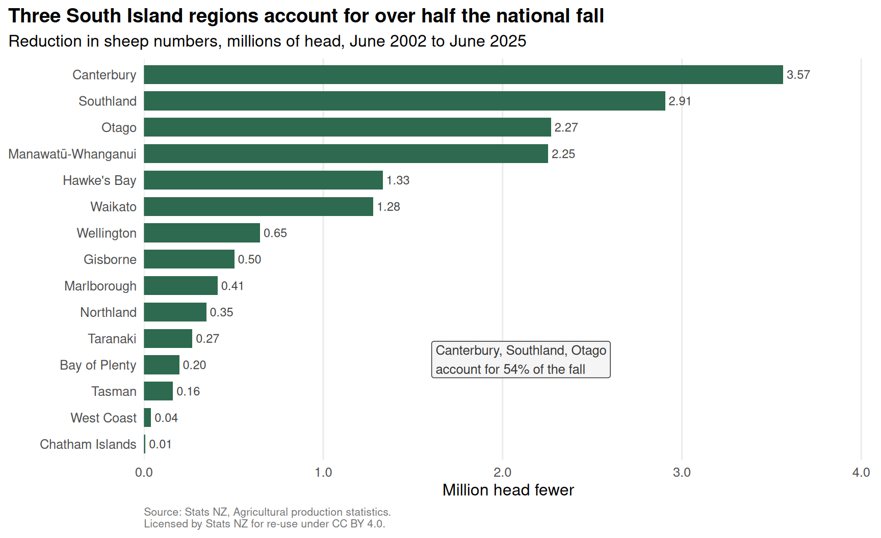
The fall is spread across the country roughly in proportion to where the sheep were. Canterbury, Southland and Otago held 50.6 percent of the 2002 flock in the 15 regions where both endpoints are published, and account for 54 percent of the fall there — 3.4 percentage points more than their size alone would give. Of the three, only Canterbury and Southland fell by more than their share of the flock. Otago is third by the narrowest of margins: it lost 2,270,557 head against Manawatū-Whanganui’s 2,254,586, a difference of 15,971 head.
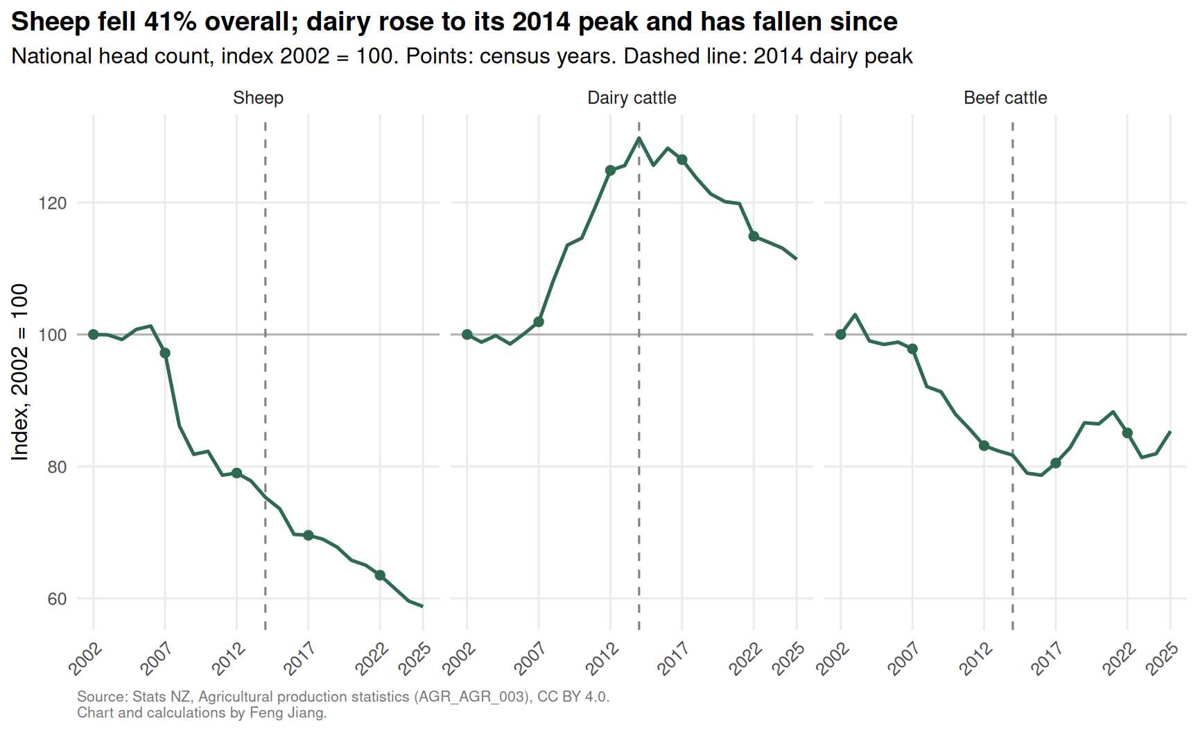
Over the same 23 years the national dairy herd rose by 588 thousand head net, while beef cattle fell by 659 thousand. The dairy net hides a 1.54 million rise to 2014 and a 0.95 million fall since.
Whether dairy fell alongside sheep depends on the window: in 7 of the 13 regions with sheep and dairy published at both ends for 2002–2025, in only 4 of 15 for 2002–2014, and in 12 of 14 for 2014–2025. The regional counts for all three windows are in Three endpoint windows.
The regional shares use the measurable regional fall as their denominator. Against the published national fall, the same three regions account for 53.6 percent. The national fall is 0.77 percent larger than the measurable regional fall because Auckland and Nelson have withheld 2025 values. The ±0.7 million sampling margin above is national and belongs to one endpoint; it says nothing about the gap between two regions. Stats NZ does not publish regional sampling errors in this table, so no uncertainty is attached to the regional shares or ranks. Otago and Manawatū-Whanganui differ by 0.4 percent of Otago’s 2025 flock and are not ranked against each other here. The top-three share depends only on which of the two is counted third: 54.0 percent with Otago, 53.9 percent with Manawatū-Whanganui.
TipTerms used on this page
Head — one animal. Every count here is a head count, not a stock unit.
Class — one of the three livestock totals used: sheep (code 6731), dairy cattle (7193) and beef cattle (7077).
Class-year — one class in one year: 3 classes × 24 years = 72.
Withheld — a cell present in the export with no value and a flag: C (confidentiality) or S (quality suppression). The data column for this is called suppressed.
Absent — a region-class-year with no row in the export at all.
Endpoint — the first or last year of a comparison window.
Measurable region — a region published (neither withheld nor absent) at both endpoints of the window in question.
Residual — the published national total minus the sum of the published regions, for one class-year.
Tier — a class-year’s residual classified by whether its region row is complete; see Data quality checks.
What this means
The common story is that sheep farms became dairy farms. In head counts, in this table, over the 2002–2025 endpoints, dairy cattle rose by 588 thousand while sheep fell by 16.3 million.
That net figure hides the shape of the series. The national dairy herd rose by 1.54 million (29.8 percent) to its 2014 peak and has fallen by 0.95 million since. Over 2002–2014, the period with the larger absolute sheep decline (−9.8 million, against −6.6 million since; the annual rates are similar, at 2.33 and 2.23 percent a year), the two moved in opposite directions. Over 2014–2025 both fell. 2014 is where the dairy herd peaks in this sample, and it was chosen after looking at the series: splitting at a peak maximises the before/after contrast by construction. 2016 is within 1.2 percent of it.
Whether the earlier dairy growth replaced the sheep in feed terms cannot be settled from head counts — see the stock-unit note below.
What these numbers do not tell you
They are head counts. They say nothing about land area, feed demand, grazing pressure, farm profitability, or what the land is used for now. A dairy cow and a sheep are not exchangeable units, and this page does not treat them as such.
The regional breakdown
Show the code
plot_dat <- measured |>mutate(region =factor(region, levels =rev(region)),millions =-change /1e6,proportional = measured_rate /100* start /1e6,group =ifelse(region %in% top3$region, "Top three", "Other regions"))p1 <-ggplot(plot_dat, aes(x = millions, y = region)) +geom_col(aes(fill = group), width =0.72) +geom_errorbar(aes(xmin = proportional, xmax = proportional),width =0.72, colour ="grey15", linewidth =0.6) +geom_text(aes(x =pmax(millions, proportional), label =sprintf("%.2f", millions)),hjust =-0.15, size =3.1, colour ="grey25") +annotate("label", x =max(plot_dat$millions) *0.9,y =nrow(plot_dat) -1.9,label =sprintf("%s:\n%.0f%% of the fall across these %d regions,\n%.1f%% of their %d flock",and_list(top3$region), top3_share, measurable, top3_base, START_YEAR),hjust =0, size =3.2, linewidth =0, fill ="grey96", colour ="grey20") +scale_fill_manual(values =c("Top three"="#1b4332", "Other regions"="#95a5a0"),guide ="none") +scale_x_continuous(labels =label_comma(accuracy =0.1),expand =expansion(mult =c(0, 0.3))) +labs(title =sprintf("Three regions account for %.0f%% of the measurable regional fall,\nand held %.1f%% of the %d flock in these regions", top3_share, top3_base, START_YEAR),subtitle =sprintf("Reduction in sheep, millions of head, June %d to June %d. Tick: fall at the %.1f%% average rate", START_YEAR, END_YEAR, measured_rate),x ="Million head fewer", y =NULL,caption =paste0(and_list(excluded), " not shown: ", END_YEAR," value withheld.\n", CAPTION) ) +theme_minimal(base_size =12) +theme(panel.grid.major.y =element_blank(),panel.grid.minor =element_blank(),plot.title.position ="plot",plot.title =element_text(face ="bold", size =12),plot.caption =element_text(colour ="grey45", hjust =0, size =8))ggsave("outputs/figures/01-regional-contribution.png", p1,width =9, height =6, dpi =200, bg ="white")p1
Figure 1: Sheep declines across the 15 regions with both endpoints published, June 2002 to June 2025. Auckland and Nelson are not shown: their 2025 values are withheld.
Auckland and Nelson are missing from that chart: each has a withheld 2025 value, so no change can be computed for them. They are excluded and counted, never imputed and never set to zero.
By percentage rather than head, the steepest declines are elsewhere: Northland (66.6 percent), Marlborough (52.3 percent), Waikato (49.3 percent) and Southland (48.8 percent), against 41.3 percent across all measurable regions.
The share of the fall taken by the three largest declines stays above half for every end year tested below; which three they are does not stay the same. Otago and Manawatū-Whanganui are all but tied, and the census-to-census window below puts Manawatū-Whanganui in the top three in place of Otago.
Show the code
measured |>transmute(Region = region,`Share of fall`=sprintf("%.1f%%", fall_share),`Share of flock`=sprintf("%.1f%%", base_share),`Difference (points)`=sprintf("%+.1f", excess_pp),`Own decline`=sprintf("%.1f%%", -pct)) |>kable(align ="lrrrr")
Table 1: Each measurable region’s share of the 2002–2025 sheep fall against its share of the 2002 flock.
Region
Share of fall
Share of flock
Difference (points)
Own decline
Canterbury
22.0%
19.8%
+2.2
46.0%
Southland
17.9%
15.2%
+2.8
48.8%
Otago
14.0%
15.6%
-1.6
37.1%
Manawatū-Whanganui
13.9%
16.7%
-2.8
34.3%
Hawke’s Bay
8.2%
9.7%
-1.4
35.1%
Waikato
7.9%
6.6%
+1.3
49.3%
Wellington
4.0%
4.6%
-0.6
35.7%
Gisborne
3.1%
4.3%
-1.2
30.0%
Marlborough
2.5%
2.0%
+0.5
52.3%
Northland
2.1%
1.3%
+0.8
66.6%
Taranaki
1.7%
1.8%
-0.1
38.7%
Bay of Plenty
1.2%
1.1%
+0.2
47.4%
Tasman
1.0%
0.9%
+0.1
45.5%
West Coast
0.2%
0.2%
+0.0
43.2%
Chatham Islands
0.1%
0.1%
-0.1
15.0%
Did dairy replace the sheep?
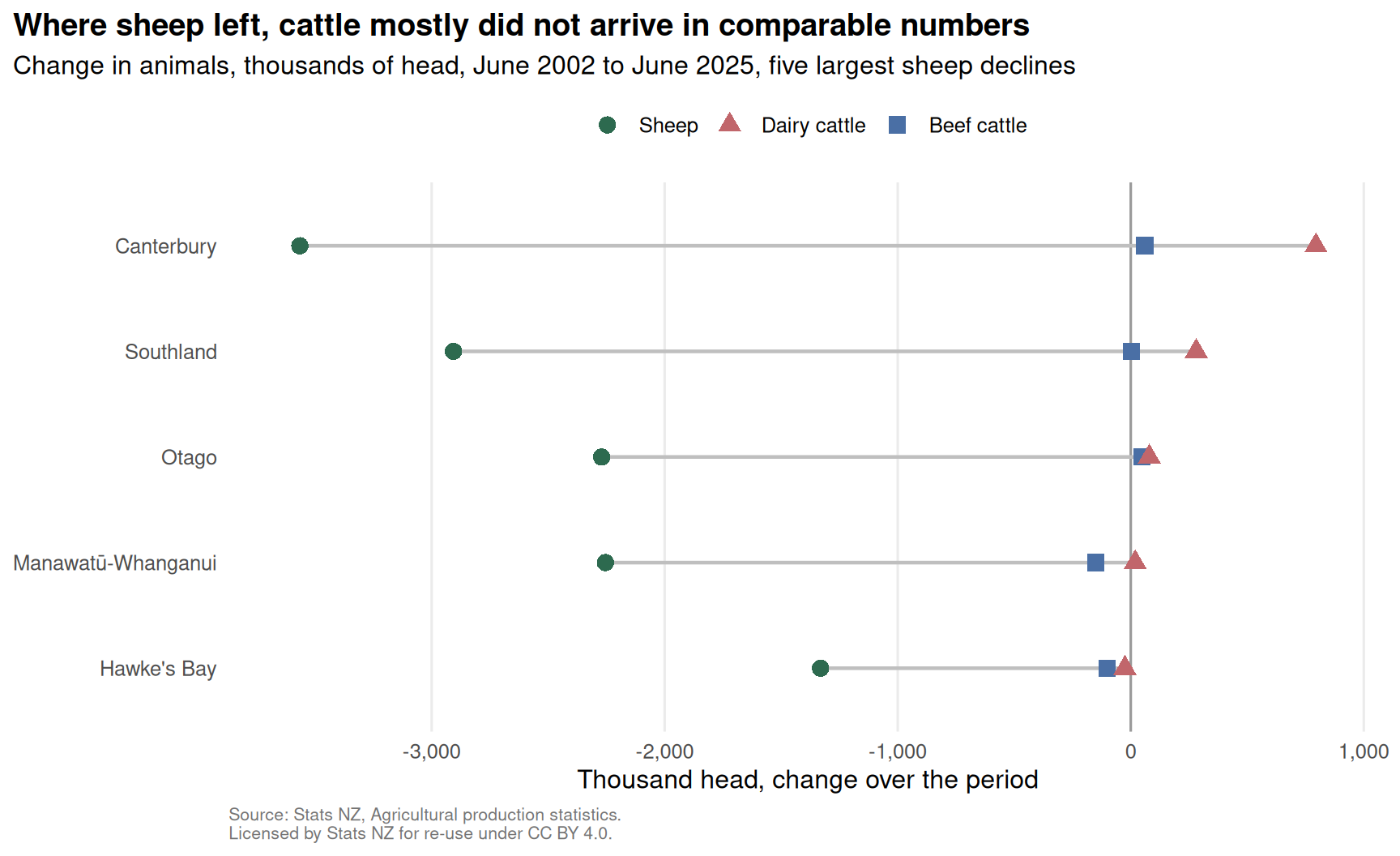
In head counts, among the five regions that lost the most sheep, only Canterbury and, to a lesser extent, Southland added dairy cattle in numbers that register against their sheep losses: 22.3 and 9.7 dairy cattle per 100 sheep lost, against at most 3.5 in the other three. Nationally, dairy grew until 2014 and has fallen since. Whether dairy replaced sheep in feed or land terms cannot be answered from this table.
Figure 2: National sheep, dairy cattle and beef cattle, indexed to 2002 = 100, June 2002 to June 2025.
Three endpoint windows
Show the code
window_counts |>transmute(Window =paste(y0, y1, sep ="–"),`Dairy fell`=paste(fell, "of", n),`Not measurable`= excluded,!!sprintf("Dairy fell, the %d regions measurable in all three", length(common)) :=paste(common_fell, "of", length(common))) |>kable(align ="lrlr")
Table 2: Regions in which dairy cattle fell, by window, among regions with sheep and dairy published at both ends.
Window
Dairy fell
Not measurable
Dairy fell, the 13 regions measurable in all three
2002–2025
7 of 13
Auckland, Wellington, Nelson and Chatham Islands
7 of 13
2002–2014
4 of 15
Nelson and Chatham Islands
2 of 13
2014–2025
12 of 14
Auckland, Wellington and Nelson
12 of 13
Each window admits the regions published at both of its own endpoints, so the three counts are not over the same regions; the last column repeats them on the 13 regions measurable in all three. The 2014–2025 count includes the Chatham Islands, which had no dairy cattle at either end and so could not have fallen.
Table 3: Published national totals for three comparison windows.
Window
Design
Class
Start head
End head
Change (head)
Change (%)
2002–2014
census → survey
Beef cattle
4,491,281
3,669,862
-821,419
-18.3
2002–2014
census → survey
Dairy cattle
5,161,589
6,698,326
+1,536,737
+29.8
2002–2014
census → survey
Sheep
39,571,837
29,803,402
-9,768,435
-24.7
2014–2025
survey → survey
Beef cattle
3,669,862
3,832,668
+162,806
+4.4
2014–2025
survey → survey
Dairy cattle
6,698,326
5,749,870
-948,456
-14.2
2014–2025
survey → survey
Sheep
29,803,402
23,252,463
-6,550,939
-22.0
2002–2022
census → census
Beef cattle
4,491,281
3,821,156
-670,125
-14.9
2002–2022
census → census
Dairy cattle
5,161,589
5,930,033
+768,444
+14.9
2002–2022
census → census
Sheep
39,571,837
25,132,697
-14,439,140
-36.5
These are published national totals, not sums with missing regions filled with zero. Splitting at 2014 separates the earlier dairy expansion from the later period; the 2002–2022 window compares two censuses. The other windows include sample-survey estimates, so their differences also carry sampling error.
A head of dairy cattle and a sheep do not require the same feed, so a head-count comparison is not a feed-equivalent one. This analysis uses total-head codes only: total sheep (6731), total dairy cattle (7193) and total beef cattle (7077). The comparisons in this section are in head counts. Whether they also hold in feed terms — stock units — is not asserted here either way: a class-specific stock-unit comparison was not attempted.
Doing one properly needs two things this analysis does not have. It needs the class-specific codes rather than the totals, because applying one adult-cow or adult-ewe coefficient to a mixed-age total assumes a herd composition the extract does not state. And it needs stock-unit coefficients from a citable source, matched to those classes. The extract carries numeric codes and no labels, so identifying the class-specific codes is itself a verification step, not a lookup.
Show the code
classes <-c("Sheep", "Dairy cattle", "Beef cattle")offset <-c("Sheep"=0.22, "Dairy cattle"=0, "Beef cattle"=-0.22)dumb <- substitution |>filter(region %in% top5_regions) |>pivot_longer(-region, names_to ="livestock_class", values_to ="change") |>mutate(y =match(region, rev(top5_regions)) + offset[livestock_class],livestock_class =factor(livestock_class, levels = classes),millions = change /1e6 )p2 <-ggplot(dumb, aes(x = millions, y = y)) +geom_vline(xintercept =0, colour ="grey60") +geom_segment(aes(x =0, xend = millions, yend = y, colour = livestock_class),linewidth =0.6, alpha =0.6) +# Shape as well as colour, so colour is not the only channel carrying the# distinction. The green and the red-brown are close under red-green colour# vision deficiency; WCAG 1.4.1 asks that colour not be used alone.geom_point(aes(colour = livestock_class, shape = livestock_class), size =3.2) +scale_colour_manual(values =c("Sheep"="#2d6a4f","Dairy cattle"="#c1666b","Beef cattle"="#4a6fa5"), name =NULL) +scale_shape_manual(values =c("Sheep"=16, "Dairy cattle"=17,"Beef cattle"=15), name =NULL) +scale_y_continuous(breaks =seq_along(top5_regions), labels =rev(top5_regions)) +scale_x_continuous(labels =label_comma(accuracy =0.1),expand =expansion(mult =0.07)) +labs(title =sprintf("Change in head counts, %d–%d, five largest sheep declines", START_YEAR, END_YEAR),subtitle ="Millions of head. Head counts are not feed-equivalent",x ="Million head, change over the period", y =NULL,caption = CAPTION ) +theme_minimal(base_size =12) +theme(panel.grid.major.y =element_blank(),panel.grid.minor =element_blank(),legend.position ="top",plot.title.position ="plot",plot.title =element_text(face ="bold"),plot.caption =element_text(colour ="grey45", hjust =0, size =8))ggsave("outputs/figures/02-substitution.png", p2,width =9, height =5.5, dpi =200, bg ="white")p2
Figure 3: Change in sheep, dairy cattle and beef cattle in the five regions that lost the most sheep, June 2002 to June 2025. Head counts are not feed-equivalent.
Table 4: Cattle gained (+) or lost (−) per 100 sheep lost, five largest sheep declines, ordered by sheep lost.
Region
Sheep lost
Dairy cattle per 100 sheep lost
Beef cattle per 100 sheep lost
Canterbury
3,565,643
+22.3
+1.7
Southland
2,906,676
+9.7
+0.1
Otago
2,270,557
+3.5
+2.2
Manawatū-Whanganui
2,254,586
+0.9
-6.6
Hawke’s Bay
1,331,249
-1.9
-7.7
Canterbury accounts for by far the largest absolute dairy increase of any region, at 795 thousand head. It is not, however, the highest ratio: West Coast gained 39 dairy cattle per 100 sheep lost, on a base so small — under 40 thousand sheep — that the ratio says more about the denominator than about land use. Hawke’s Bay and Manawatū-Whanganui lost sheep and at least one cattle class. A negative figure in this table means that class of animal declined as well.
Data quality checks
Five rules run over the analysis table on every render.
Table 5: Validation rules on the analysis table. Items: cells checked. nNA: cells where the rule could not be evaluated.
Rule
Items
Passes
Fails
Not evaluable (nNA)
head_non_negative
1397
1397
0
0
value_iff_suppressed
1397
1397
0
0
region_label_present
1397
1397
0
0
no_duplicate_cells
1397
1397
0
0
census_year_reported
1397
1388
9
0
Four pass. The fifth fires 9 times, and that is a finding rather than a defect. census_year_reported asserts that a census year — a full-coverage collection, with no sampling error to exceed a threshold — should not have withheld cells. It is wrong. Census years do withhold cells, because withholding is about confidentiality and imputation quality, not about coverage. The rule earns its place by being falsified. It sees only flagged cells, so a cell absent from the export is invisible to it: 9 is a lower bound on census-year withholding, not a count of it.
Three of the four passing rules cannot fail on anything the loader returns, because ingestion already stops on a negative count, a value without a flag or a flag without a value, and an unmapped region code. On the real data their zeroes restate the ingestion contract; the corrupted copy below is what shows that the rules themselves fire.
Showing that the rules can fail
An all-green table is not evidence. A reader cannot tell from it whether the rules are sound or merely too loose to fire. So the same five rules are also run against a deliberately corrupted copy of the analysis table: one negative count, one withheld cell filled with a zero, one census-year value removed, one region label deleted, and one duplicated row.
Show the code
results |>select(rule, `real data`= fails) |>left_join(select(results_corrupted, rule, `corrupted copy`= fails),by ="rule") |>kable(align ="lrr", col.names =c("Rule", "Fails on real data","Fails on corrupted copy"))
Table 6: The same rules on the real data and on a deliberately corrupted copy.
Rule
Fails on real data
Fails on corrupted copy
head_non_negative
0
1
value_iff_suppressed
0
1
region_label_present
0
1
no_duplicate_cells
0
2
census_year_reported
9
10
Each corruption moves exactly one rule. no_duplicate_cells moves by two because a duplicate makes both members of the pair non-unique, and census_year_reported moves from 9 to 10 because it already fails 9 times on the real data. The corrupted rows are chosen at distinct indices and the function asserts as much, so no single corruption can be counted twice.
The more interesting result is in the reconciliation: the published national total against the sum of the regions.
Table 7: Sheep: sum of published regions against the published national total, by year.
Year
Region rows present
Region rows absent
Regions withheld
Sum of regions
Published national
Residual (head)
Residual %
2002
17
0
0
39,571,837
39,571,837
0
0.000
2003
15
2
0
39,408,419
39,552,113
143,694
0.363
2004
15
2
0
39,198,830
39,271,137
72,307
0.184
2005
16
1
0
39,824,732
39,879,668
54,936
0.138
2006
15
2
0
39,980,941
40,081,594
100,653
0.251
2007
17
0
0
38,460,477
38,460,477
0
0.000
2008
16
1
0
33,767,565
34,087,864
320,299
0.940
2009
16
1
0
32,312,249
32,383,589
71,340
0.220
2010
17
0
0
32,562,612
32,562,612
0
0.000
2011
17
0
0
31,132,328
31,132,329
1
<0.001
2012
17
0
0
31,262,715
31,262,715
0
0.000
2013
17
0
0
30,786,762
30,786,761
-1
<0.001
2014
17
0
0
29,803,402
29,803,402
0
0.000
2015
17
0
0
29,120,829
29,120,827
-2
<0.001
2016
17
0
0
27,583,672
27,583,673
1
<0.001
2017
17
0
1
27,506,969
27,526,537
19,568
0.071
2018
17
0
2
27,202,153
27,295,749
93,596
0.343
2019
17
0
2
26,535,840
26,821,846
286,006
1.066
2020
17
0
1
26,008,537
26,028,935
20,398
0.078
2021
17
0
4
25,174,579
25,732,889
558,310
2.170
2022
17
0
1
25,113,843
25,132,697
18,854
0.075
2023
17
0
1
24,338,666
24,359,267
20,601
0.085
2024
17
0
1
23,363,016
23,583,001
219,985
0.933
2025
17
0
2
22,997,178
23,252,463
255,285
1.098
There are 17 expected regional rows for sheep in each year. An absent row is different from a present row whose value is withheld. The exported coverage table records both: suppression_rate divides withheld rows by present rows, and suppression_rate_all_regions divides them by 17. Neither treats absent rows as withheld or as zero-valued livestock counts.
The residual column is reported in head as well as in percent on purpose. At a base of 30 million, a percentage rounded to three decimal places renders a discrepancy of one animal as 0.000, which would let the table appear to support a stronger claim than the numbers do; non-zero residuals below that resolution are shown as <0.001.
A residual is arithmetic on published cells, but when a single region is withheld it equals that region’s value to within a head or two. Stats NZ does not apply secondary suppression to the national totals, so this is a property of the published table; the page still does not report residuals for class-years carrying the confidentiality flag C, or describe any residual as a named region’s value. outputs/reconciliation.csv carries every residual, because the port check compares it.
Across all three livestock classes the residual separates into three tiers.
Table 8: Every class-year, classified by whether its region row is complete and how closely it reconciles.
Tier
Class-years
Largest absolute residual (head)
Exact
10
0
Fully published, off by a few head
12
2
Incomplete region row
50
701,526
In 10 of the 22 class-years where all 17 regions are published and nothing is withheld, the regions sum to the published national total exactly, to the head.
Completeness is checked before the residual, so a class-year with an incomplete region row is never Exact however well it reconciles. That matters here: 11 class-years reconcile to zero, 1 more than the Exact tier contains, because 1 class-year with an incomplete region row happens to reconcile exactly anyway.
In 12 further fully-published class-years the residual never exceeds 2 head, on bases between 3.5 and 31.1 million. I cannot attribute that from published data. It is consistent with the national aggregate being rounded independently of the regional cells, but I have not been able to source that and do not assert it. It is not input perturbation: every one of these class-years falls between 2008 and 2016, before perturbation was introduced in 2017, and the 2 fully-published class-years from 2017 on have residuals of 0.
Every residual larger than that — and the next smallest is 507 head — belongs to a year whose region row is incomplete, because a region is withheld or because a region row is absent from that year’s export.
What the one-head residuals are not is an artefact of this analysis. The same discrepancy appears between cells that this analysis never sums. Adding the two published island totals and comparing them against the published national total — three aggregate cells, always published, never withheld — gives a difference of one head in 14 of the 72 class-years, and never more than 1.
Table 9: Class-years in which the two published island totals do not sum to the published national total.
Year
Class
North Island
South Island
Sum
Published NZ
Difference
2003
Beef cattle
3,400,859
1,225,759
4,626,618
4,626,617
-1
2005
Beef cattle
3,249,727
1,173,898
4,423,625
4,423,626
1
2006
Beef cattle
3,258,533
1,180,602
4,439,135
4,439,136
1
2014
Beef cattle
2,604,422
1,065,439
3,669,861
3,669,862
1
2018
Beef cattle
2,620,089
1,101,174
3,721,263
3,721,262
-1
2019
Beef cattle
2,707,287
1,182,710
3,889,997
3,889,996
-1
2020
Beef cattle
2,636,865
1,245,702
3,882,567
3,882,566
-1
2023
Beef cattle
2,501,041
1,152,992
3,654,033
3,654,034
1
2004
Dairy cattle
3,787,210
1,365,281
5,152,491
5,152,492
1
2005
Dairy cattle
3,731,709
1,355,468
5,087,177
5,087,176
-1
2009
Dairy cattle
3,796,485
2,064,292
5,860,777
5,860,776
-1
2018
Dairy cattle
3,816,099
2,569,441
6,385,540
6,385,541
1
2004
Sheep
18,734,141
20,536,997
39,271,138
39,271,137
-1
2009
Sheep
16,077,872
16,305,716
32,383,588
32,383,589
1
So the one-head discrepancies are a property of the published table, not of the join. That does not explain them, but it does locate them.
Withholding is not constant over time
Show the code
status_labels <-c("C"="C flag: confidentiality (before 2017)","S"="S flag: quality suppression","Absent"="Absent from the export: no row")p3 <- status_by_year |>filter(status !="Published") |>mutate(status =factor(unname(status_labels[status]), levels =rev(unname(status_labels)))) |>ggplot(aes(x = year, y = rate)) +annotate("rect", xmin = CENSUS_YEARS -0.5, xmax = CENSUS_YEARS +0.5,ymin =-Inf, ymax =Inf, fill ="grey93") +geom_col(aes(fill = status), width =0.7) +scale_fill_manual(values =setNames(c("#e07a5f", "#6c8ea4", "#c9c3b6"),unname(status_labels)), name =NULL,breaks =unname(status_labels)) +scale_x_continuous(breaks =sort(unique(c(START_YEAR, CENSUS_YEARS, END_YEAR))),limits =c(START_YEAR -1, END_YEAR +1)) +scale_y_continuous(labels =label_percent(scale =1), limits =c(0, NA),expand =expansion(mult =c(0, 0.05))) +guides(fill =guide_legend(nrow =2)) +labs(title =sprintf("Rows are absent until %d; confidentiality flags appear in %s; quality suppression from %d, peaking in %d",max(absent_years), and_list(c_years), min(s_years), peak_row$year),subtitle =sprintf("Percentage of the %d expected region-by-class cells not published: sheep, dairy and beef cattle. Shaded: census years", cells_per_year),x =NULL, y ="Cells not published",caption = CAPTION ) +theme_minimal(base_size =12) +theme(panel.grid.major.x =element_blank(),panel.grid.minor =element_blank(),legend.position ="top",plot.title.position ="plot",plot.title =element_text(face ="bold", size =11),plot.caption =element_text(colour ="grey45", hjust =0, size =8))ggsave("outputs/figures/03-suppression-rate.png", p3,width =9, height =5, dpi =200, bg ="white")p3
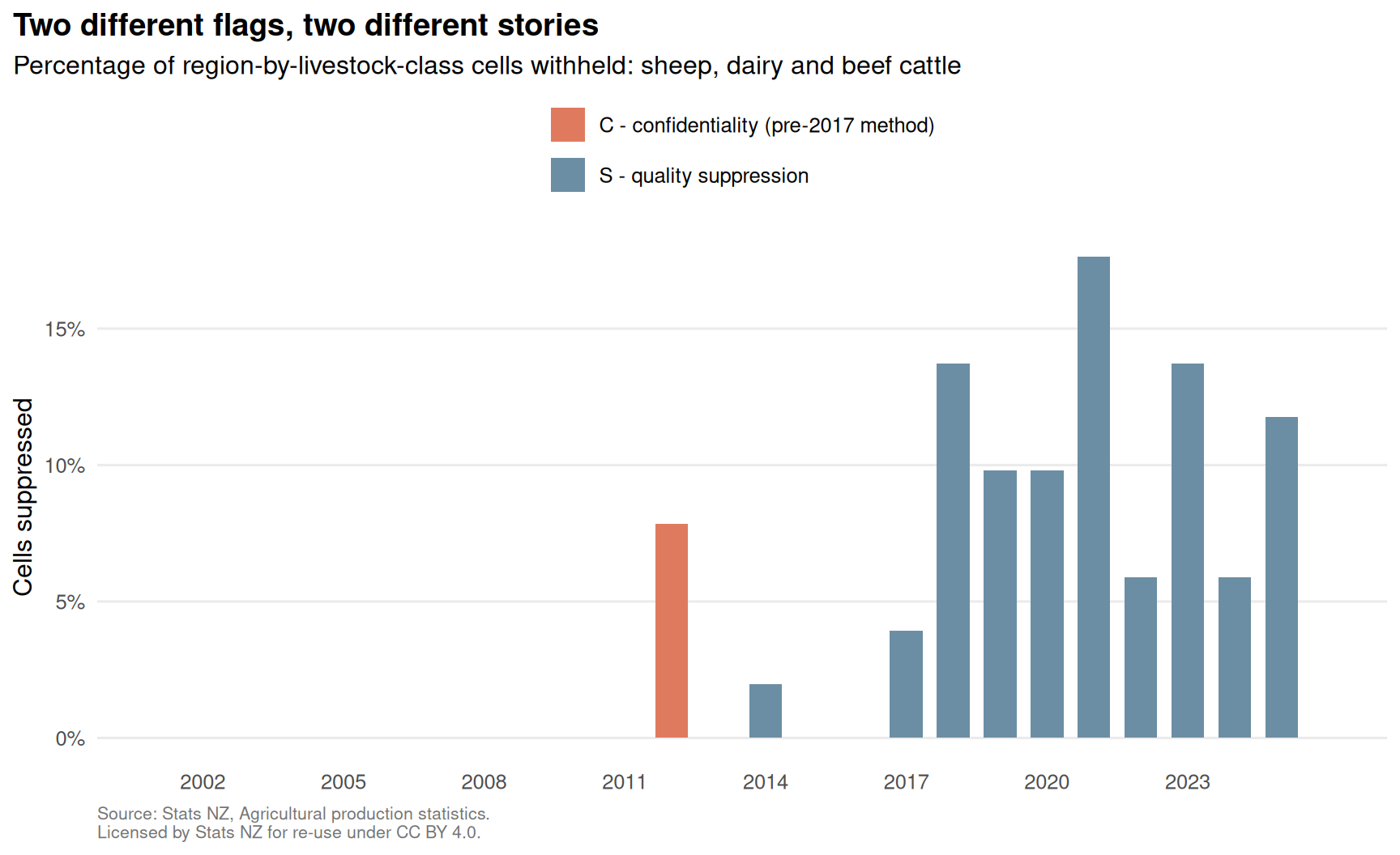
Figure 4: Share of the 51 expected region-by-class cells each year that are withheld with a flag, or absent from the export.
Reading that chart as a single rising trend would be wrong, and the OBS_STATUS column is what makes the difference visible. Two flags are in use, they are not the same mechanism, and before either appears the export does something else entirely.
Before 2012, cells are left out rather than flagged. From 2002 to 2011 no cell carries a flag, but the export has fewer rows than the full grid of regions and classes; from 2012 on it is complete. An absent row is not a zero. In 21 of the 22 class-years whose region row is incomplete without any flag, the published regions fall short of the published national total, by between 507 and 320,299 head, so the animals were counted and not shown; the exception reconciles exactly, as it would if the missing region had none of that class. And the cells that carry C in 2012 look like the cells that were absent before: across all 44 livestock codes, 51 of the 51 regional C cells of 2012 had been absent from the export in at least one earlier year, on average 8.2 of the 10 years from 2002 to 2011. The change in 2012 is a change in the export’s format; it is not evidence that nothing was withheld before it, and this chart is not a trend in withholding before 2012.
The C flag is confidentiality suppression. Among the three livestock classes used here it appears in 2012 and in no other year. Checked across every one of the 44 livestock codes in the raw extract, it appears in 2012–2016 and never after 2016.
That is what the published methodology predicts. Stats NZ states that prior to 2017, figures affected by the confidentiality provisions were denoted by C, and that since 2017 confidentiality has instead been implemented by an input perturbation method that adds noise at individual farm level, so output figures no longer have to be replaced with C. The flag stops in the file in the same year the method changed.
The S flag is quality suppression, applied where sampling errors or imputation levels are high. It appears in 2014, then every year from 2017 to 2025, peaking at 17.6 percent of cells in 2021. The census years hold few S cells — 2 in 2017 and 3 in 2022, against a median of 6 in the survey years since 2017 — which is consistent with a census removing the sampling-error branch of the rule while leaving the imputation branch. 2 census years are far too few to establish it. All 5 census-year S cells in this table are Nelson.
So the 2012 spike is not a quality problem. All 4 withheld cells that year carry C, not S.
One of the two regions this analysis has to drop is explained in the published methodology rather than guessed at. Sampling error could not be calculated for Nelson because only one responding unit was observed in each sampled stratum, and at least two are needed to estimate a within-stratum variance. Auckland, the other dropped region, is simply withheld, with no reason published.
Method
One table, one vintage. Stats NZ table AGR_AGR_003, Livestock Numbers by Regional Council, dataflow STATSNZ:AGR_AGR_003(1.0), final vintage, downloaded once and committed with its SHA-256. Full provenance is in data-raw/SOURCE.md.
Codes verified before code was written. The extract carries numeric codes and no labels. Sheep, dairy cattle and beef cattle were each confirmed against the published June 2024 national figures before any analysis was run. The LIVESTOCK codelist holds 44 entries that nest inside one another; adding all 44 national totals for 2024 gives 115.7 million, against 33.1 million for the three verified totals alone. Only those three codes are used.
Aggregates are separated, not summed.AREA codes 10, 19 and 20 are the North Island, South Island and New Zealand totals. They are flagged in the analysis table and excluded from every regional sum. The extract publishes no area labels at all, only numeric codes that are this table’s own rather than SSGA23 codes; region names here follow the Statistical standard for geographic areas 2023 (SSGA23), including macrons, which differ from the older spellings the codelist still displays in Aotearoa Data Explorer.
Withheld cells stay withheld. A withheld cell becomes NA and carries a flag. It is never filled with zero and never dropped. Regions missing either endpoint are excluded from the change calculation and counted in the text.
Reconciliation is reported, not asserted. No fixed tolerance is set between the regional sum and the published total. The residual is computed for every year and published above.
Quantitative claims are computed or cited, and the two are different things. Numbers that come from the data — in the prose, the figure and table captions and the figures’ alternative text — are expressions evaluated at render time against the analysis table. Qualitative claims that depend on the data (for example, that every measurable region declined) are asserted in the code, so a new vintage that breaks one stops the render instead of leaving the sentence stale. Numbers from Stats NZ’s published methodology — sample size, eligible population, response rate, imputation level, relative sampling error, the GST threshold — cannot be computed from an aggregate extract; they are typed, and each is attributed under Sources for the methodological statements. The analysis window, the census years, the 2014 split and the five-year minimum window are design constants, set once in R/load.R, R/checks.R and the setup code of this page.
Release schedule
This analysis uses the final vintage throughout. Up to and including the 2024 survey, Stats NZ published a provisional release in mid-December and a final release in mid-May of the following year. From the 2025 survey those two were replaced by a single final release in mid-April.
Survey design
The reference period is the year ended 30 June. Censuses were held in 2002, 2007, 2012, 2017 and 2022, with annual sample surveys in the intervening years. The sample is stratified by regional council area, ANZSIC06 group and size group. The 2025 survey drew 24,600 geographic locations from an estimated eligible population of 45,800; note that a geographic location is the statistical unit and is not the same thing as a farm.
The series starts at 2002 because Stats NZ states that the population for the 2002 census and subsequent surveys differs from that of earlier agricultural censuses and surveys, and that figures from 2002 onward may not be directly comparable with previous years. That is also why the 1994 observation carried in the same table is excluded here. There was no agricultural production survey at all in 1997, 1998 or 2001.
Values for non-respondents are imputed by random hot deck imputation, with the imputation class formed from regional council area, ANZSIC06 group and production data from previous years. This matters more than it may appear: for the 2025 survey Stats NZ reports that 30 percent of the total sheep estimate was imputed, against a relative sampling error of 3 percent at 95 percent confidence. The response rate for the 2025 final release was 72.1 percent. The collection is run by Stats NZ in partnership with the Ministry for Primary Industries.
The headline window is not design-matched
2002 is a census and 2025 is a sample survey, so the headline differences a full-coverage count against an estimate that carries both sampling error and a 30 percent imputation rate. Stats NZ publishes both years in the same table, but the comparison is still an asymmetry, and this report carries the is_census_year flag through the analysis table precisely so that it can be checked rather than assumed.
The census-to-census window that avoids the asymmetry is 2002 to 2022:
Show the code
rbind(data.frame(Window =sprintf("%d–%d, census to sample survey (headline)", START_YEAR, END_YEAR),Regions = headline$regions,Fall =fmt(headline$fall),`Top three share`=sprintf("%.1f%%", headline$share),`Their share of the flock`=sprintf("%.1f%%", headline$base_share),`The three regions`= headline$top3,check.names =FALSE),data.frame(Window =sprintf("%d–%d, census to census (design-matched)", START_YEAR, LAST_CENSUS),Regions = matched$regions,Fall =fmt(matched$fall),`Top three share`=sprintf("%.1f%%", matched$share),`Their share of the flock`=sprintf("%.1f%%", matched$base_share),`The three regions`= matched$top3,check.names =FALSE)) |>kable(align ="lrrrrl")
Table 10: The headline window against the design-matched census-to-census window.
Window
Regions
Fall
Top three share
Their share of the flock
The three regions
2002–2025, census to sample survey (headline)
15
16,195,353
54.0%
50.6%
Canterbury, Southland, Otago
2002–2022, census to census (design-matched)
16
14,446,905
55.6%
51.2%
Canterbury, Southland, Manawatū-Whanganui
The design-matched window is measurable across 1 more region, because Auckland is published in 2022 and withheld in 2025. The share is similar: a fall of 14.4 million head with the three largest decliners accounting for 55.6 percent, against 51.2 percent of the flock. The three are not the same: Manawatū-Whanganui replaces Otago. The share is robust; the list is not.
The 2025 endpoint is used in the headline because it is the most recent published figure, not because it is the better-matched one.
What was excluded, and why
Territorial authority geography — the surveys are designed to produce results to regional council level and the censuses to territorial authority level, so no annual series exists below the region.
Horticulture — not collected in 2004, 2006, 2008, 2010, 2013, 2015, 2016, 2018, 2021, 2023 or 2025, which is most of this window.
Forestry production — Stats NZ no longer collects or compiles forestry production statistics; they are published by MPI. Stats NZ does still collect forestry land use. The 2025 release also notes that additional National Exotic Forest Description data has been received and that revisions to earlier land use and forestry statistics, especially for 2016 to 2021, are planned.
Pre-2002 data — the population change described above, plus the absence of any survey in 1997, 1998 and 2001.
A choropleth map — a sorted bar chart answers “which regions contributed most” and a map does not, because a map encodes land area rather than magnitude. Canterbury, Otago and Southland are also three of the largest regions by area, which is precisely the confound a map would introduce.
A second data set — the question is answerable inside one table, and every extra source adds provenance to defend without adding evidence.
Implications for output design
Three observations follow from the checks above, and they concern the shape of the output rather than the sheep.
Regional council is the only geography available annually; territorial authority exists only in census years, so any sub-regional time series is structurally unavailable rather than merely unpublished. Withholding has exceeded ten percent of cells in 2 of the last 4 years, and it is not spread evenly. Nelson and the Chatham Islands account for 56 percent of all withheld cells in this table between them, Auckland for a further 10 percent, and 7 other regions for the rest.
Two different grounds are at work, and it is worth separating them. Nelson and the Chathams are withheld persistently — they hold the two smallest livestock populations in the table — which makes their trends unusable. (By sheep alone, averaged over the years each is published, the second smallest is West Coast, published in 21 of the 24 years: being small and being withheld are not the same thing.) Auckland is withheld only at scattered points including the 2025 endpoint, which is what removes it from this analysis’ change calculation while leaving most of its series intact. Auckland is not a small region, and by sheep it is not even among the smallest: its last published count is larger than Northland’s or West Coast’s. Being withheld and being small are related here but not the same thing, and an output that conflated them would mislead.
A suppression-aware grouping that pooled the persistently withheld regions would preserve more signal than withholding them one at a time does. And the alternating census-and-survey design makes every regional series in this table structurally uneven, which belongs on the output rather than being left for a user to discover from a reconciliation residual.
There is also a class of question this data cannot answer at all: anything at farm level, or any breakdown finer than what is published. The access route for those questions is approved microdata under the Five Safes framework, which I have not used here.
Sources for the methodological statements
Every statement about the collection above was read on the page cited here, not carried over from secondary summaries. Pages read 4 September 2026.
Statement
Source
Census years 2002, 2007, 2012, 2017, 2022, with sample surveys in between
Statements that could not be sourced on those pages are not made anywhere in this report.
Limitations
Non-census years are sample estimates. I have not recomputed their sampling errors and I have applied no weighting of my own. A year-on-year movement in a single small region should not be read as real change, and regional rankings separated by small margins — such as Otago and Manawatū-Whanganui — should not be read as ranked at all.
Withheld cells are retained as NA and counted. Two regions are excluded from the 2002–2025 change entirely for that reason.
The sheep-to-cattle comparisons are ratios of head counts. They are not claims about stocking rate, feed demand, land use or emissions.
The frame is Stats NZ’s Business Register, which is built on GST registration. The compulsory registration level is $60,000, and Stats NZ describes coverage of units below that level as “partial and unquantifiable”.
Imputation is large. Stats NZ reports 30 percent of the 2025 national sheep estimate as imputed. That national rate does not establish the imputation rate for any individual region or another year; this extract does not provide those rates, and this analysis does not adjust the published estimates. Whether hot-deck imputation biases changes towards zero has not been assessed here.
Since 2017, confidentiality has been implemented by input perturbation, which adds noise at individual farm level. Its size is not published on the pages cited here, so it is not quantified; it is present in every year from 2017 on.
The endpoints are of different collection designs. 2002 is a census and 2025 is a sample survey. The is_census_year flag is carried through the analysis table for exactly this reason, and the design-matched comparison is reported under Survey design.
Choosing the start and end years is a choice, and the two halves of the headline survive it differently. See the sensitivity analysis below.
How much does the start year matter?
Recomputing the headline statistic from every start year that leaves a window of at least 5 years — 2002 to 2020 — against the same 2025 endpoint. The five-year minimum is an analysis choice to focus on longer windows. Starts in 2021–2024 are excluded, so the sensitivity conclusions apply only to the windows shown:
Show the code
sensitivity |>transmute(`Start year`=ifelse(start %in% CENSUS_YEARS,paste0(start, " (census)"), as.character(start)),`Regions measurable`= regions,`Gross fall (head)`=fmt(fall),`Net fall (head)`=fmt(net_fall),`Top three share`=sprintf("%.1f%%", share),`Their share of the flock`=sprintf("%.1f%%", base_share),`The three regions`= top3 ) |>kable(align ="lrrrrrl")
Table 11: The headline statistic from every start year, 2002 to 2020, against the 2025 endpoint.
Start year
Regions measurable
Gross fall (head)
Net fall (head)
Top three share
Their share of the flock
The three regions
2002 (census)
15
16,195,353
16,195,353
54.0%
50.6%
Canterbury, Southland, Otago
2003
14
16,098,121
16,098,121
54.6%
52.1%
Canterbury, Southland, Manawatū-Whanganui
2004
14
15,924,689
15,924,689
52.0%
49.8%
Canterbury, Southland, Otago
2005
14
16,540,440
16,540,440
52.9%
51.4%
Canterbury, Southland, Manawatū-Whanganui
2006
14
16,738,228
16,738,228
52.1%
51.1%
Canterbury, Southland, Manawatū-Whanganui
2007 (census)
15
15,168,071
15,168,071
52.9%
51.3%
Canterbury, Southland, Manawatū-Whanganui
2008
14
10,700,360
10,690,974
48.3%
49.9%
Canterbury, Southland, Manawatū-Whanganui
2009
14
9,111,028
9,101,375
48.3%
48.7%
Southland, Manawatū-Whanganui, Otago
2010
15
9,329,065
9,318,046
48.4%
48.6%
Southland, Manawatū-Whanganui, Otago
2011
15
7,919,219
7,901,455
52.4%
53.4%
Manawatū-Whanganui, Canterbury, Otago
2012 (census)
15
8,053,801
8,053,801
51.0%
49.3%
Otago, Southland, Manawatū-Whanganui
2013
15
7,590,781
7,571,115
52.5%
49.7%
Otago, Southland, Manawatū-Whanganui
2014
15
6,581,367
6,581,367
55.9%
50.3%
Otago, Southland, Manawatū-Whanganui
2015
15
5,902,153
5,874,290
59.4%
51.0%
Otago, Manawatū-Whanganui, Southland
2016
15
4,408,959
4,379,565
53.7%
49.6%
Otago, Manawatū-Whanganui, Southland
2017 (census)
15
4,268,875
4,256,717
57.0%
50.0%
Southland, Manawatū-Whanganui, Otago
2018
13
4,108,545
4,076,041
55.5%
50.0%
Otago, Manawatū-Whanganui, Southland
2019
14
3,608,010
3,576,665
53.7%
47.3%
Otago, Manawatū-Whanganui, Hawke’s Bay
2020
14
2,939,552
2,870,621
58.3%
54.5%
Otago, Manawatū-Whanganui, Canterbury
Gross fall sums losses only in the declining regions with both endpoints published; it is the denominator for Top three share. Net fall subtracts gains in other measurable regions. Neither is the published national fall, because some regional endpoints are withheld or absent. For 2002–2025 every measurable region declined, so the gross and net regional falls are both 16,195,353 head against a published national fall of 16,319,374, a gap of 0.77 percent, as set out at the top of this page.
Across the 19 start years the three largest-declining regions account for between 48 and 59 percent of the gross regional fall, while holding between 47 and 54 percent of the starting flock. The narrower claim “over half” does not hold for every start year: the share is below 50 percent for 2008, 2009 and 2010.
Which three regions they are is not robust. Manawatū-Whanganui is in the top three in 17 of the 19 windows, Otago in 14, Southland in 16, and Canterbury in only 9 — 2002, 2003, 2004, 2005, 2006, 2007, 2008, 2011 and 2020. Canterbury dominates the window this report uses because its decline is concentrated in the early years: from a start year of 2009 on, it is in the top three only for 2011 and 2020.
That is worth stating plainly, because Canterbury is the region this report names most often. It leads the 2002–2025 window, and it is the one region where the substitution story carries weight. It is not a permanent feature of the data.
And the end year?
Holding the start at 2002 and moving the end instead, from 2007 to 2025. The measurable regions change from window to window, so the shares do not share a denominator; the last column names the regions each window excludes.
Show the code
end_sensitivity |>transmute(`End year`=ifelse(end %in% CENSUS_YEARS,paste0(end, " (census)"), as.character(end)),`Regions measurable`= regions,`Top three share`=sprintf("%.1f%%", share),`Their share of the flock`=sprintf("%.1f%%", base_share),`The three regions`= top3,`Not measurable`=ifelse(excluded =="", "—", excluded) ) |>kable(align ="lrrrll")
Table 12: The headline statistic from 2002 to every end year, 2007 to 2025.
End year
Regions measurable
Top three share
Their share of the flock
The three regions
Not measurable
2007 (census)
17
70.4%
36.6%
Canterbury, Southland, Marlborough
—
2008
16
67.5%
50.6%
Canterbury, Southland, Otago
Tasman
2009
16
62.3%
50.2%
Canterbury, Southland, Otago
Chatham Islands
2010
17
60.6%
50.1%
Canterbury, Southland, Otago
—
2011
17
58.5%
50.1%
Canterbury, Southland, Otago
—
2012 (census)
17
59.6%
51.2%
Canterbury, Southland, Manawatū-Whanganui
—
2013
17
59.0%
51.2%
Canterbury, Southland, Manawatū-Whanganui
—
2014
17
58.1%
51.2%
Canterbury, Southland, Manawatū-Whanganui
—
2015
17
59.0%
51.2%
Canterbury, Southland, Manawatū-Whanganui
—
2016
17
57.8%
51.2%
Canterbury, Southland, Manawatū-Whanganui
—
2017 (census)
16
56.2%
50.1%
Canterbury, Southland, Otago
Nelson
2018
15
59.7%
51.4%
Canterbury, Southland, Manawatū-Whanganui
West Coast and Chatham Islands
2019
15
60.1%
51.8%
Canterbury, Southland, Manawatū-Whanganui
Auckland and Chatham Islands
2020
16
56.8%
51.4%
Canterbury, Southland, Manawatū-Whanganui
West Coast
2021
13
58.6%
52.5%
Canterbury, Southland, Manawatū-Whanganui
Auckland, Bay of Plenty, West Coast and Chatham Islands
2022 (census)
16
55.6%
51.2%
Canterbury, Southland, Manawatū-Whanganui
Nelson
2023
16
54.6%
51.3%
Canterbury, Southland, Manawatū-Whanganui
Chatham Islands
2024
16
54.8%
51.7%
Canterbury, Southland, Manawatū-Whanganui
Auckland
2025
15
54.0%
50.6%
Canterbury, Southland, Otago
Auckland and Nelson
From every end year the three largest declines take more of the fall than they held of the flock, by between 3.1 and 33.8 percentage points. Canterbury and Southland are in the top three for every end year; the third place moves between Manawatū-Whanganui, Marlborough and Otago.
Ethics
This analysis uses published regional aggregates only. No microdata and no IDI access is involved, so the Five Safes framework does not apply to it.
Stats NZ lists Tatauranga Umanga Māori among the internal users of this collection, and signed the Mana Ōrite Relationship Agreement with the Data Iwi Leaders Group of the National Iwi Chairs Forum in October 2019. Any Māori-specific cut of this data therefore sits inside an established relationship between Stats NZ and iwi Māori. It does not sit with an unaffiliated analyst working from published aggregates, which is why this report does not attempt one and does not characterise the terms of that agreement.
Reproduce
The full command sequence — restoring the pinned packages, the ingestion and helper tests, regenerating the CSVs and rendering this page — is in the README.
R/load.R reads the SHA-256 recorded in data-raw/SOURCE.md and stops unless the extract’s bytes match it, then tidies the extract; R/checks.R runs the rules and both reconciliations; index.qmd produces this page, the figures and outputs/key-figures.csv.
Both sets of outputs are committed. A clean checkout that runs the documented commands must reproduce the CSVs byte for byte. The figures are regenerated as well, but their bytes can differ with the platform’s fonts and graphics device, so they are checked for existence rather than compared.
That claim is checked rather than asserted. A GitHub Actions workflow runs the commands on a clean Ubuntu runner for every pull request and every push to main, and weekly, and fails if any committed CSV differs. On main, the site it rendered and verified is the one deployed to GitHub Pages, so what you are reading is the output of a build that passed.
It earned its place on the first run, by failing. The extract arrives from the SDMX endpoint with CRLF line endings and the recorded SHA-256 is the hash of those bytes, but Git had normalised them to LF on commit. The hash gate therefore passed on the Windows machine this was written on, where checkout restores the CRLFs, and would have stopped every clone on Linux or macOS at the first line of R/load.R. .gitattributes now marks data-raw/*.csv as -text so Git leaves those bytes alone.
The general point is worth more than the fix: a single machine cannot see a whole class of defect, because the thing that hides the defect is the same thing that makes the analysis run. Only a second platform could find that one.